Binding and scoping
Lecture 5. How a program names its values, and how far each name reaches.
Programming Languages Lab · University of Pisa
Vincenzo Ciancia, CNR-ISTI
vincenzo.ciancia@isti.cnr.it · github.com/vincenzoml/PLDW
Lecture 4, exercises 1 and 2
Power and named constants
Exercise 1 · A power operator
evaluate_string("2^3")      # 8
evaluate_string("2*3")      # 6
The assignment, from Lecture 4
- In
domains.py, add"^"to theOPterminal and bind it topowerincreate_initial_env. - Check that
evaluatedid not need any change.
Exercise 1: the solution
OP: "+" | "-" | "*" | "/" | "%" | "^"

env = bind(env, "^", power)

evaluate_string("2^3")      # 8
Two lines, and evaluate does not change.
Exercise 2 · Named constants
evaluate_string("ten * 2")       # 20
evaluate_string("ten + ten")     # 20
evaluate_string("eleven")        # ValueError
The assignment, from Lecture 4
- Bind
tento10in the initial environment: it is aDValtoo. - Add an
IDENTIFIERterminal, a rule for it inmono, a nodeVar(name)and its case inevaluate. - Write the equation for
Varfirst, then the code. - What should
+ + 1andten(1, 2)do? Which stage reports each error?
Exercise 2: the solution
mono: ground | var | paren
var: IDENTIFIER
IDENTIFIER: /[a-zA-Z_][a-zA-Z0-9_]*/

@dataclass(frozen=True)
class Var:
    name: str

case Tree(data="var",
          children=[Token(type="IDENTIFIER", value=name)]):
    return Var(name=name)
A name is one more kind of mono: it can stand wherever a number can.
IDENTIFIER is a letter or _, followed by letters, digits and _: the same rule as for Python names.
The parse tree has a node var, which becomes a Var in the AST.
The equation for a name
\( ⟦x⟧\rho = \rho(x) \)
case Var(name):
    meaning = lookup(env, name)
    if callable(meaning):
        raise ValueError(
            f"{name} is an operator, not a value")
    return meaning
The value of a name is what the environment says it stands for.
The check is the mirror of the one for operators: a name used as a value must stand for a number.
+ + 1 and ten(1, 2) are syntax errors: the parser rejects them, before any environment is involved.
Who puts ten in the environment?
def create_initial_env() -> Environment:
    ...
    env = bind(env, "ten", 10)
    return env

evaluate_string("ten * 2")     # 20
evaluate_string("eleven")      # ValueError: Undefined identifier: eleven
Only the Python program that runs the interpreter. The program written in our language can use names, but cannot create them.
Today the language gets a construct that adds a name to the environment: let.
The code of this lecture is in code/lesson-05/: binding.py and scoping.py.
Binding
Giving names to values
Why names
(17 * 23 + 4) * (17 * 23 + 4) - (17 * 23 + 4)

let n = 17 * 23 + 4 in n * n - n
The same expression written three times is three chances to make a mistake, and three times the work.
The second line computes it once, gives the result a name, and uses the name.
It also says something to the reader: these three are the same thing.
let, in three parts
let  x  =  3  in  x + 1
     │     │      └── the body: where x can be used
     │     └── the definition: its value is given to x
     └── the name
The value of the whole expression is the value of the body, computed in an environment where x stands for 3. Here, 4.
The syntax comes from ISWIM, a language designed by Peter Landin in 1966, through ML. Haskell, OCaml and F# still write it this way.
Binding is not assignment
BINDING
let x = 3 in ... makes a new environment where x stands for 3. It is valid in the body, and nowhere else. Nothing that existed before is changed.
ASSIGNMENT
x = 3 in Python changes what x stands for, from now on. Code that read x before and reads it again later sees two different values.
Our language has binding only. A name, once bound, stands for the same value in all of its body.
Assignment needs memory, which can change while the program runs: Lecture 6.
The same program, two answers
Our language
let x = 3 in
  let f = x + 1 in
    let x = 10 in
      f                 # 4
Python
x = 3
f = lambda: x + 1
x = 10
f()                     # 11
The second let x makes a new x; the x that f was computed from is still 3. The second x = 10 changes the only x there is, and f reads it when it is called.
Syntax
The grammar of let
The grammar
grammar = r"""
    ?expr: let | arith
    let: "let" IDENTIFIER "=" expr "in" expr
    ?arith: bin | mono
    bin: arith OP mono
    mono: ground | var | paren
    paren: "(" expr ")"
    ground: NUMBER
    var: IDENTIFIER

    NUMBER: /[0-9]+/
    OP: "+" | "-" | "*" | "/" | "%"
    IDENTIFIER: /(?!(let|in)\b)[a-zA-Z_][a-zA-Z0-9_]*/

    %import common.WS
    %ignore WS
"""
The rules of Lecture 4 move one level down, into arith. Above them, an expression is a let or an arithmetic expression.
The definition and the body of a let are expr: they can contain other lets.
Since let is above arith, it cannot be an operand: 1 + let x = 2 in x is a syntax error. Write 1 + (let x = 2 in x).
"let", "=" and "in" are anonymous strings: they do not appear in the parse tree.
Where the body ends
let x = 1 in x + 2         3
(let x = 1 in x) + 2       3
let x = 1 in (x + 2)       3

2 + let y = 3 in y         syntax error
2 + (let y = 3 in y)       5
The body goes as far to the right as it can. In the first line it is x + 2, not x.
The left side of bin is an arith, so it cannot be a let: let x = 1 in x followed by + 2 is not a way to read the first line. There is one parse tree only.
A let inside arithmetic needs parentheses.
OCaml accepts 2 + let y = 3 in y. We chose a smaller grammar with no ambiguity; the price is some parentheses.
Reserved words
IDENTIFIER: /(?!(let|in)\b)[a-zA-Z_][a-zA-Z0-9_]*/
Without the first part, let and in would also match IDENTIFIER, and let in = 3 in in would be a program.
(?!...) means "not followed by": a name cannot start with the word let or the word in. \b is the end of a word, so inside and let1 are still names.
Python has 35 reserved words: if, def, lambda, ... Try lambda = 3 in Python.
The AST
@dataclass(frozen=True)
class Let:
    name: str
    definition: Expression
    body: Expression


type Expression = Number | Var | BinaryExpression | Let


case Tree(data="let",
          children=[Token(type="IDENTIFIER", value=name),
                    definition, body]):
    return Let(name=name,
               definition=transform_parse_tree(definition),
               body=transform_parse_tree(body))
One new node, with the three parts of a let.
The name is a string, not an expression: let 3 = x in ... is not a program.
A parse tree and its AST
let
  x
  mono
    ground	1
  bin
    mono
      var	x
    +
    mono
      ground	2
Let(name='x',
    definition=Number(value=1),
    body=BinaryExpression(op='+',
                          left=Var(name='x'),
                          right=Number(value=2)))
The parse tree of let x = 1 in x + 2, from parser.parse(...).pretty(), and the AST built from it.
Semantics
What let means
Two new equations
\( ⟦x⟧\rho = \rho(x) \)
\( ⟦\mathtt{let}\ x = e_1\ \mathtt{in}\ e_2⟧\rho = ⟦e_2⟧\big(\rho[x \mapsto ⟦e_1⟧\rho]\big) \)
- The definition \( e_1 \) is computed in \( \rho \), the environment the
letis in. - The body \( e_2 \) is computed in a different environment: \( \rho \) with one more name.
This is the first equation where the environment on the right is not the one on the left. Until today, \( \rho \) was passed down unchanged.
The evaluator
def evaluate(ast: Expression, env: Environment) -> EVal:
    match ast:
        case Number(value):
            return value
        case Var(name):
            meaning = lookup(env, name)
            if callable(meaning):
                raise ValueError(
                    f"{name} is an operator, not a value")
            return meaning
        case BinaryExpression(op, left, right):
            ...                       # as in Lecture 4
        case Let(name, definition, body):
            value = evaluate(definition, env)
            return evaluate(body, bind(env, name, value))
The Let case is the equation, line by line.
Compute the definition in env. Build a new environment with bind. Compute the body in it.
This is the use of bind announced in Lecture 4: env is not changed, and the code after the let still sees it as it was.
Equations and code, side by side
| equation | Python |
|---|---|
| ⟦x⟧ρ = ρ(x) | case Var(name): ... lookup(env, name) |
| ⟦e₁⟧ρ | value = evaluate(definition, env) |
| ρ[x ↦ ⟦e₁⟧ρ] | bind(env, name, value) |
| ⟦e₂⟧(ρ[x ↦ ...]) | evaluate(body, bind(...)) |
As in Lecture 4, each equation is one case, and the recursive calls are on the children of the node.
let x = 1 in
  let y = x + 1 in
    x * y
evaluate(Let('x', 1, Let('y', x + 1, x * y)), ρ0)
  evaluate(Number(1), ρ0)                         1
  ρ1 = bind(ρ0, "x", 1)
  evaluate(Let('y', x + 1, x * y), ρ1)
    evaluate(x + 1, ρ1)                           2
    ρ2 = bind(ρ1, "y", 2)
    evaluate(x * y, ρ2)
      lookup(ρ2, "x")                             1
      lookup(ρ2, "y")                             2
      multiply(1, 2)                              2
\( \rho_0 \) is the initial environment, with the five operators. Each let builds a new environment on top of the previous one.
The chain, while computing x * y
lookup(ρ2, "x") goes from ρ2 to ρ1, which answers 1. lookup(ρ2, "*") goes all the way to ρ0.
The same picture as in Lecture 4. Then the chain was built by Python code; now it is built by the program.
Scope
Where a name is valid
The scope of a binding
let x = 3 in x + 1
    ─        ─────
    binds    scope of x
The scope of a binding is the part of the program where the name refers to it. For let x = e₁ in e₂, the scope of x is e₂, and only e₂.
The equation says it: \( \rho[x \mapsto ...] \) is used for \( e_2 \) and for nothing else.
The scope is a part of the text of the program. It can be found by reading the program, without running it.
Outside the scope
(let x = 1 in x) + x
The second x is outside the parentheses, so outside the body: it is not in the scope of the let.
Undefined identifier: x
When the let is done, evaluate goes back to the environment it had, which does not contain x. Nothing needs to be removed.
The definition is not in the scope
let x = x + 1 in x                Undefined identifier: x

let x = 1 in let x = x + 10 in x * 2       22
In let x = x + 1 in ..., the x of the definition is computed in \( \rho \), before x is bound.
If an outer x exists, the definition uses it: in the second line, the inner x is 1 + 10.
A let whose definition sees its own name is a recursive binding. Recursive functions need it; we will come back to it.
Shadowing
In let x = 1 in let x = x + 10 in x * 2 there are two bindings of x. In x * 2, the inner one wins.
The outer binding is shadowed: it still exists, but in the inner body it cannot be reached by its name.
lookup stops at the first environment that knows the name. Shadowing needs no code of its own.
Shadowing ends with the scope
let x = 5 in (let x = 1 in x) + x                6
(let x = 2 in x * x) + (let x = 3 in x * x)      13
In the first line the inner x is 1 inside the parentheses; after them, x is 5 again.
In the second line the two x are unrelated: each let builds its own environment from the initial one.
With assignment, x = 1 inside the parentheses would destroy the 5. With binding, the old environment is still there.
Free and bound
x + y                    free: x, y
let x = 1 in x + y       free: y
let x = x in x           free: x
let y = 2 in 3           free: none
An occurrence of a name is bound if it is in the scope of a let for that name; otherwise it is free.
The free names are those the expression needs from outside: its value depends on what the environment says about them.
In the third line, the first x after = is free, the last one is bound.
Free variables, in Python
def free_variables(ast: Expression) -> frozenset[str]:
    match ast:
        case Number(_):
            return frozenset()
        case Var(name):
            return frozenset({name})
        case BinaryExpression(_, left, right):
            return free_variables(left) | free_variables(right)
        case Let(name, definition, body):
            return (free_variables(definition)
                    | (free_variables(body) - {name}))
A function with the same structure as evaluate: one case per node, recursion on the children.
The Let case follows the scope: the definition counts in full, the body without the bound name.
It does not need an environment and does not compute anything: it only reads the text. A program with no free names is closed, and can be run in the initial environment without Undefined identifier errors.
Scoping
Static and dynamic
When is the definition computed?
Our let computes the definition first, then the body: it is eager. Another choice: bind the name to the definition itself, not computed, and compute it each time the name is used.
let z = 1 / 0 in 7
Eager: Division by zero. The other way: 7, because z is never used.
This is the idea behind the lazy evaluation of Haskell. The code of this part is in scoping.py.
Then a question comes up
let x = 5 in
  let f = x + 10 in
    let x = 42 in
      f
When f is used, its definition x + 10 is computed. Which x?
STATIC · 15
The x visible where f was defined: the environment of its let.
DYNAMIC · 52
The x visible where f is used: the environment at that moment.
The equations
\( ⟦\mathtt{let}\ x = e_1\ \mathtt{in}\ e_2⟧\rho = ⟦e_2⟧\big(\rho[x \mapsto (e_1, \rho)]\big) \)
let binds x to a pair: its definition \( e_1 \) and the environment \( \rho \) of the let. When x is used, with \( \rho(x) = (e, \rho') \):
STATIC
\( ⟦x⟧\rho = ⟦e⟧\rho' \)
Compute \( e \) in \( \rho' \), the environment saved at the let.
DYNAMIC
\( ⟦x⟧\rho = ⟦e⟧\rho \)
Compute \( e \) in \( \rho \), the environment where x is used. \( \rho' \) is ignored.
The pair \( (e, \rho') \) is a closure, as in Lecture 4.
In real languages
Python: static
x = 1
def f():
    return x
def g():
    x = 2
    return f()
g()        # 1
bash: dynamic
x=1
f() { echo $x; }
g() { local x=2; f; }
g          # 2
In Python, x in f is the one visible where f is written. In bash, it is the one of whoever called f.
Early Lisp and Emacs Lisp scope dynamically too. Almost every language designed since the 1980s scopes statically.
Why static scoping won
- The meaning of a name can be found by reading the text around it. With dynamic scoping, it depends on the path the program took to get there.
- Renaming a bound name, consistently, never changes the result. With dynamic scoping, renaming
xingchanges whatfprints. free_variablestells, before running, which names a closed program needs. With dynamic scoping a name can be found at run time in a caller.
The difference really matters with functions, which are code that runs later, far from where it was written. Functions come in a later lecture, with closures as their values.
Summary
Names in your language
The decisions of today
| decision | alternative | why |
|---|---|---|
| binding | assignment | no memory needed; a name means one thing in its whole scope |
let at the top level of an expression | let anywhere, as in OCaml | one parse tree only; some parentheses |
| reserved words | keywords usable as names | a simpler parser, clearer programs |
| definition outside its scope | recursive binding | let x = x + 1 uses the outer x |
| eager | delayed | each definition computed once |
| static scoping | dynamic scoping | names can be understood by reading the text |
let: all the changes
PARSER
?expr: let | arith
let: "let" IDENTIFIER "=" expr "in" expr
mono: ground | var | paren
var: IDENTIFIER
AST
@dataclass(frozen=True)
class Let:
    name: str
    definition: Expression
    body: Expression
EVALUATE
case Let(name, definition, body):
    value = evaluate(definition, env)
    return evaluate(body,
        bind(env, name, value))
Everything else is as in Lecture 4. The full code is in code/lesson-05/binding.py.
Where we are
A program can now add names to the environment, with let. Two new equations, two new cases in evaluate, and bind as it was in Lecture 4.
The scope of a name is a part of the text. Static scoping keeps it that way; dynamic scoping makes it depend on the run.
Names cannot change value yet. Lecture 6, state and commands, adds memory: a name stands for a location, and the content of the location can change.
Exercises
Your turn
Exercise 1 · Predict, then run
let a = 2 in let b = a * a in let a = b + 1 in a * b
let x = 3 in (let y = x in y * x) + (let x = 1 in x)
let n = 10 in let m = n % 3 in let n = n / m in n - m
(let p = 4 in p) * (let q = p in q)
Today's interpreter: code/lesson-05/binding.py
Level 1 of 4
- For each line, write the value, or the error, before running it.
- For each occurrence of a name, say which
letbinds it, or that it is free. - Check with
evaluate_stringandfree_variablesinbinding.py.
Exercise 2 · Check before running
run("let x = 1 in x + y")
# ValueError: free names: y

run("let x = 1 in x + 1")     # 2
Level 2 of 4
- Write
run(text): parse, callfree_variables, and evaluate only if the program is closed. - Give an example where the check reports an error that evaluation alone would not reach.
- Which stage of the interpreter does this check belong to: parser, transform, or a new one?
Exercise 3 · Several names at once
let x = 1, y = 2 in x + y          3
let x = 1, y = x + 1 in x * y      ?
Level 3 of 4
- Extend the grammar, the AST and
evaluateto allow several bindings in onelet. - Two choices for the second line: each definition sees the names before it, or no definition sees any of them. Write the equation for each.
- Can you implement it without a new AST node, by transforming into nested
Lets?
Exercise 4 · A language for text
"ab" * 3                          ababab
"programming"[0:7]                program
upper("ciao") + nl + reverse("ciao")
                                  CIAO
                                  oaic
let s = "Pisa" in s + nl + ("-" * length(s))
                                  Pisa
                                  ----
let w = "na" in (w * 8 + nl) * 2 + upper("batman")
Level 4 of 4 · a longer one
A new language, built from binding.py: a program computes a text.
| construct | meaning |
|---|---|
"..." | a text, written between double quotes |
a + b | the two texts, one after the other |
a * n | a repeated n times |
reverse(a), upper(a), lower(a) | backwards, in capitals, in small letters |
nl | a text with one newline in it |
a[i:j] | the characters from position i to j, excluded, as in Python |
let x = e₁ in e₂ | as today |
Exercise 5 · extra
Images in Python
Exercise 5 · A language for images
print(circle & square)
                       the circle, in front of the square
print(circle | mirror(circle))
                       two circles, side by side
let c = scale(circle, 0.5) in
  print((c | c) / (c | c))
                       four small circles, in a grid
let bg = load("sky.png") in
  print(circle & bg)
Extra · a language of images
A new language, built from binding.py: a program computes an image.
| construct | meaning |
|---|---|
circle, square | the two example images, 512 × 512 |
load("file.png") | an image read from a file |
a & b | a in front of b: over |
a | b, a / b | side by side, a on top of b: beside, above |
mirror(a), scale(a, f) | flipped left to right, resized by f |
print(a) | opens a window with a; its value is a |
let x = e₁ in e₂ | as today |
The next slides give the Python primitives, in images.py. print calls show.
The library: Pillow
# once, in the terminal of VS Code
# pip install pillow

from pathlib import Path
from PIL import Image, ImageDraw, ImageOps
The standard library of Python has no module for images. Pillow is the one almost everybody uses.
Three of its modules are enough: Image to load, save and combine, ImageDraw to draw shapes, ImageOps for ready-made transformations.
pathlib is in the standard library: a Path is a file name that knows how to join folders, HERE / "red_circle.png". Pillow is now in requirements.txt.
Load and save
HERE = Path(__file__).parent

def load(path: Path) -> Image.Image:
    with Image.open(path) as image:
        return image.convert("RGBA")

def save(image: Image.Image, path: Path) -> None:
    image.save(path)

circle = load(HERE / "red_circle.png")
print(circle.size, circle.mode)
print(circle.getpixel((206, 206)))
print(circle.getpixel((10, 10)))
(512, 512) RGBA
(220, 40, 40, 200)
(0, 0, 0, 0)
convert("RGBA") gives every image the same form, whatever the file was: four numbers per pixel.
with closes the file when the block ends; convert has already made a copy in memory.
save chooses the format from the extension: .png keeps transparency, .jpg does not.
Pixels with alpha
| pixel | R, G, B | alpha | meaning |
|---|---|---|---|
(220, 40, 40, 200) | red | 200 | red, slightly transparent |
(40, 80, 220, 160) | blue | 160 | blue, more transparent |
(0, 0, 0, 0) | any | 0 | nothing: fully transparent |
(255, 255, 255, 255) | white | 255 | white, fully opaque |
Each number goes from 0 to 255. The fourth one, alpha, says how much the pixel covers what is behind it: 0 not at all, 255 completely.
In the slides, the transparent parts are drawn on a grey checkerboard.
Drawing the two examples
SIZE = 512

def red_circle() -> Image.Image:
    image = Image.new("RGBA", (SIZE, SIZE), (0, 0, 0, 0))
    draw = ImageDraw.Draw(image)
    draw.ellipse((56, 56, 356, 356), fill=(220, 40, 40, 200))
    return image

def blue_square() -> Image.Image:
    image = Image.new("RGBA", (SIZE, SIZE), (0, 0, 0, 0))
    draw = ImageDraw.Draw(image)
    draw.rectangle((176, 176, 456, 456), fill=(40, 80, 220, 160))
    return image
Image.new makes a transparent image; ImageDraw draws on it.
The four numbers of ellipse and rectangle are the corners of a box: left, top, right, bottom. The circle and the square overlap in the middle.
The files are already in code/images/; these functions are how they were made.
Compositing: one image over another
def over(front: Image.Image,
         back: Image.Image) -> Image.Image:
    return Image.alpha_composite(back, front)

over(circle, square).getpixel((300, 300))
# (194, 46, 66, 235)


alpha_composite puts the second image on top of the first. over takes them in the order we read them: front, then back.
Where both are present, the front lets a part of the back show through. With alpha between 0 and 1:
\( \alpha = \alpha_f + \alpha_b (1 - \alpha_f) \)
The order matters: over is not commutative. The two images on the left differ only in the middle.
A position, and a scale
def over(front: Image.Image, back: Image.Image,
         x: int = 0, y: int = 0) -> Image.Image:
    result = back.copy()
    result.alpha_composite(front, dest=(x, y))
    return result

def scale(image: Image.Image, factor: float) -> Image.Image:
    width = max(1, round(image.width * factor))
    height = max(1, round(image.height * factor))
    return image.resize((width, height),
                        Image.Resampling.LANCZOS)

small = scale(circle, 0.5)          # 256 × 256
over(small, square, 256, 256)

With x and y, the top-left corner of front goes at that point of back. What falls outside back is cut away.
scale multiplies width and height by factor; LANCZOS is a way to compute the new pixels that keeps edges smooth.
This over is the one in the file. With x = y = 0 it gives the same result as the previous slide. Pillow does not accept a negative position.
More operations
def beside(left: Image.Image, right: Image.Image) -> Image.Image:
    result = Image.new("RGBA",
                       (left.width + right.width,
                        max(left.height, right.height)),
                       (0, 0, 0, 0))
    result.paste(left, (0, 0))
    result.paste(right, (left.width, 0))
    return result

def mirror(image: Image.Image) -> Image.Image:
    return ImageOps.mirror(image)

def fade(image: Image.Image, factor: float) -> Image.Image:
    r, g, b, a = image.split()
    a = a.point(lambda v: round(v * factor))
    return Image.merge("RGBA", (r, g, b, a))
beside makes an image wide enough for both and pastes them in. above, in the file, does the same vertically.
mirror flips left to right. fade splits the four channels, multiplies alpha by factor, and puts them back.
point applies a function to every pixel of a channel: a function passed as a value, as in Lecture 4.
Every operation returns a new image
paste and the method alpha_composite change the image they are called on. That is why beside pastes onto a new image, and over draws on a copy of back.
Then over, scale, beside, mirror and fade are pure functions: the images they receive are not changed, and the same arguments give the same image.
Exercise 5 · The results

print(circle & square)
print(circle | mirror(circle))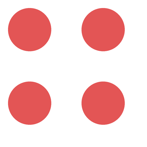
let c = scale(circle, 0.5) in print((c | c) / (c | c))
let bg = load("sky.png") in print(circle & bg)What each print shows. A solution is in code/images/imagelang.py: run it with --show to open the windows.